Theoretical basics of Inorganic chemistry

Introduction. Around the 5^th century BC, Greek philosopher Democritus invented the concept of the atom (from Greek meaning “indivisible”). The atom, eternal, constant, invisible and indivisible, represented the smallest unit and the building block of all matter. Democritus suggested that the varieties of matter and changes in the universe arise from different relations between these most basic constituents. He illustrated the concept of atom by arguing that every piece of matter could be cut to an end until the last constituent is reached.

Today the word atom is used to identify the basic component of molecules that create all matter, but it is known that the atom itself is made of particles even more fundamental, some of which are elementary. The first theoretical and experimental models of the structure of matter came as late as the 19^th century, which is the time marked as the beginning of modern science. At that time a more empirical approach, mainly in chemistry, opened a new era of scientific investigations.

The work of Democritus remained known through the ages in writings of other philosophers, mainly Aristotle. Modern Greece has honored Democritus as a philosopher and the originator of the concept of the atoms through their currency; the 10-drachma coin, before Greek currency was replaced with the euro, depicted the face of Democritus on one side, and the schematic of a lithium atom on the other.

This chapter introduces the structure of atoms and describes atomic models that show the evidence for the existence of atoms and electrons [13, p. 1].

 

Atomic models. The cannonball atomic model. All matter on Earth is made from a combination of 90 naturally occurring different atoms.

 

Early in the 19^th century, scientists began to study the decomposition of materials and noted that some substances could not be broken down past a certain point (for instance, once separated into oxygen and hydrogen, water cannot be broken down any further). These primary substances are called chemical elements.

 

By the end of the 19^th century it was implicit that matter can exist in the form of a pure element, chemical compound of two or more elements or as a mixture of such compounds. Almost 80 elements were known at that time and a series of experiments provided confirmation that these elements were composed of atoms.

 

This led to a discovery of the law of definite proportions: two elements, when combined to create a pure chemical compound, always combine in fixed ratios by weight.

 

For example, if element A combines with element B, the unification creates a compound AB. Since the weight of A is constant and the weight of B is constant, the weight ratio of these two will always be the same. This also implies that two elements will only combine in the defined proportion; adding an extra quantity of one of the elements will not produce more of the compound.

 

Example 3.1: The law of definite proportion

Carbon (C) forms two compounds when reacting with oxygen (O): carbon monoxide (CO) and carbon dioxide (CO₂).

 

1g of C + 4/3 g of O → 2 1/3 g of CO; 1 g of C + 8/3 g of O → 3/2 g of CO₂

 

The two compounds are formed by the combination of a definite number of carbon atoms with a definite number of oxygen atoms. The ratio of these two elements is constant for each of the compounds (molecules): C:O = 3:4 for CO and C:O = 3:8 for CO₂.

The first atomic theory with empirical proofs for the law of definite proportion was developed in 1803 by the English chemist John Dalton (1766–1844). Dalton conducted a number of experiments on gases and liquids and concluded that, in chemical reactions, the amount of the elements combining to form a compound is always in the same proportion.

He showed that matter is composed of atoms and that atoms have their own distinct weight. Although some explanations in Dalton’s original atomic theory are incorrect, his concept that chemical reactions can be explained by the union and separation of atoms (which have characteristic properties) represents the foundations of modern atomic physics. In his two-volume book, New System of Chemical Philosophy, Dalton suggested a way to explain the new experimental chemistry. His atomic model described how all elements were composed of indivisible particles which he called atoms (he depicted atoms like cannonballs, figure 3.1) and that all atoms of a given element were exactly alike.

This explained the law of definite proportions. Dalton further explained that different elements have different atoms and that compounds were formed by joining the atoms of two or more elements.

 

In 1811, Amadeo Avogadro, conte di Quaregna e Ceretto (1776–1856), postulated that equal volumes of gases at the same temperature and pressure contain the same number of molecules. Sadly, his hypothesis was not proven until 2 years after his death at the first international conference on chemistry held in Germany in 1860 where his colleague, Stanislao Cannizzaro, showed the system of atomic and molecular weights based on Avogadro’s postulates.

 

Example 3.2: Avogadro’s law

As shown in Example 3.1, the ratio of carbon and oxygen in forming CO₂ is 3:8. Here is the explanation of this ratio: since a single atom of carbon has the same mass as 12 hydrogen atoms, and two oxygen atoms have the same mass as 32 hydrogen atoms, the ratio of the masses is 12:32 = 3:8. This shows that the description of the reaction is independent of the units used since it is the ratio of the masses that determines the outcome of a chemical reaction.

Thus, whenever you see wood burning in a fire, you should know that for every atom of carbon from the wood, two oxygen atoms from the air are combined to form CO₂; the ratio of masses is always 12:32.

It follows that there must be as many carbon atoms in 12 g of carbon as there are oxygen atoms in 16 g of oxygen. This measure of the number of atoms is called a mole. The mole is used as a convenient measure of an amount of matter, similarly as “a dozen” is a convenient measure of 12 objects of any kind. Thus, the number of atoms (or molecules) in a mole of any substance is the same. This number is called Avogadro’s number (NA) and its value was accurately measured in the 20th century as 6.02 × 10²³ atoms or molecules per mole.

For example, the number of moles of hydrogen atoms in a sample that contains 3.02 × 10²¹ hydrogen atoms is

 

Moles of H atoms = 3,02×10²¹ atoms H/6,02×10²³atoms/mole = 5.01×10^-3 moles H [13, p. 2]

 

 

Figure 3.1 Cannonball atomic model (John Dalton, 1803)

 

The Plum Pudding Atomic Model. Shortly before the end of the 19^th century, a series of new experiments and discoveries opened the way for new developments in atomic and subatomic (nuclear) physics. In November 1895, Wilhelm Roentgen (1845– 1923) discovered a new type of radiation called X-rays, and their ability to penetrate highly dense materials. Soon after the discovery of X-rays, Henri Becquerel (1852–1908) showed that certain materials emit similar rays independent of any external force. Such emission of radiation became known as radioactivity.

During this same time period, scientists were extensively studying a phenomenon called cathode rays. Cathode rays are produced between two plates (a cathode and an anode) in a glass tube filled with the very low-density gas when an electrical current is passed from the cathode to the high-voltage anode. Because the glowing discharge forms around the cathode and then extends toward the anode, it was thought that the rays were coming out of the cathode. The real nature of cathode rays was not understood until 1897 when Sir Joseph John Thomson (1856–1940) performed experiments that led to the discovery of the first subatomic particle, the electron. The most important aspect of his discovery is that the cathode rays are the stream of particles. Here is the explanation of his postulate: from the experiment he observed that cathode rays were always deflected by an electric field from the negatively charged plate inside the cathode ray tube, which led him to conclude that the rays carried a negative electric charge. He was able to determine the speed of these particles and obtain a value that was a fraction of the speed of light (one tenth the speed of light, or roughly 30,000 km/s or 18,000 mi/s). He postulated that anything that carries a charge must be of material origin and composed of particles. In his experiment, Thomson was able to measure the charge-to-mass ratio, e/m, of the cathode rays; a property that was found to be constant regardless of the materials used. This ratio was also known for atoms from electrochemical analysis, and by comparing the values obtained for the electrons he could conclude that the electron was a very small particle, approximately 1,000 times smaller than the smallest atom (hydrogen). The electron was the first subatomic particle identified and the fastest small piece of matter known at that time.

In 1904, Thomson developed an atomic model to explain how the negative charge (electrons) and positive charge (speculated to exist since it was known that the atoms were electrically neutral) were distributed in an atom. He concluded that the atom was a sphere of positively charged material with electrons spread equally throughout like raisins in a plum pudding. Hence, his model is referred to as the plum pudding model, or raisin bun atom as depicted in figure 3.2. This model could explain

·         The neutrality of atoms

 

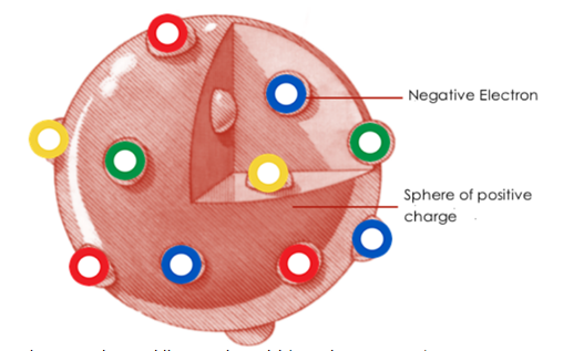
Figure 3.2 Plum pudding atomic model (J. J. Thomson, 1904)

 

·         The origin of electrons

·         The origin of the chemical properties of elements. However, his model could not answer questions regarding

·         Spectral lines (according to this model, radiation emitted should be monochromatic; however, experiments with hydrogen shows a series of lines falling into different parts of the electromagnetic spectrum)

·         Radioactivity (nature of emitted rays and their origin in the atom). Scattering of charged particles by atoms

Thomson won the Nobel Prize in 1906 for his discovery of the electron. He worked in the famous Cavendish Laboratory in Cambridge and was one of the most influential scientists of his time. Seven of his students and collaborators won Nobel Prizes, among them his son who, interestingly, won the Nobel Prize for proving the electron is a wave [13, p. 4].

 

The Planetary Atomic Model. Disproof of Thomson’s Plum Pudding Atomic Model. Thomson’s atomic model described the atom as a relatively large, positively charged, amorphous mass of a spherical shape with negatively charged electrons homogeneously distributed throughout the volume of a sphere, the sizes of which were known to be on the order of an Ångström (1 Å = 10^-8 cm = 10^-10 m). In 1911 Geiger and Marsden carried out a number of experiments under the direction of Ernest Rutherford (1871–1937) who received the Nobel Prize in chemistry in 1908 for investigating and classifying radioactivity. He actually did his most important work after he received the Nobel Prize and the 1911 experiment unlocked the hidden nature of the atom structure.

Rutherford placed a naturally radioactive source (such as radium) inside a lead block as shown in figure 3.3. The source produced α particles which were collimated into a beam and directed toward a thin gold foil. Rutherford hypothesized that if Thomson’s model was correct then the stream of α particles would pass straight through the foil with only a few being slightly deflected as illustrated in figure 3.4. The “pass through” the atom volume was expected because the Thomson model postulated a rather uniform distribution of positive and negative charges throughout the atom. The deflections would occur when the positively charged α particles came very close to the individual electrons or the regions of positive charges. As expected, most of the α particles went through the gold foil with almost no deflection. However, some of them rebounded almost directly backward – a phenomenon that was not expected (figure 3.5).

 

 

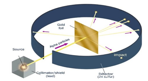
Figure 3.3 Schematics of Rutherford’s experiment (1911)

 

 

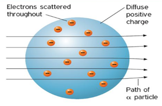
Figure 3.4 Expected scattering of α particles in Rutherford’s experiment

 

 

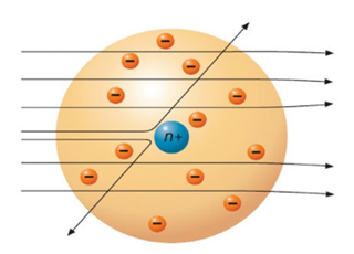
Figure 3.5 Actual scattering of α particles in Rutherford’s experiment

 

Rutherford explained that most of the α particles pass through the gold foil with little or no divergence not because the atom is a uniform mixture of the positive and negative charges but because the atom is largely empty space and there is nothing to interact with the α particles. He explained the large scattering angle by suggesting that some of the particles occasionally collide with, or come very close to, the “massive” positively charged nucleus that is located at the center of an atom. It was known at the time that the gold nucleus had a positive charge of 79 units and a mass of about 197 units while the α particle had a positive charge of 2 units and a mass of 4 units. The repulsive force between the α particle and the gold nucleus is proportional to the product of their charges and inversely proportional to the square of the distance between them. In a direct collision, the massive gold nucleus would hardly be moved by the α particle. The diameter of the nucleus was shown to be ~1/105 the size of the atom itself, or ~10−13 m. Clearly these ideas defined an atom very different from the Thomson’s model.

Ernest Solvay (1838–1922), a Belgian industrial chemist, who made a fortune from the development of a new process to make washing soda (1863), was known for his generous financial support to science, especially physics research. Among the projects he financially supported, was a series of international conferences, known as the Solvay conferences. The First Solvay Conference on Physics was held in Brussels in 1911 and it was attended by the most famous scientists of the time. Rutherford was one of them; he presented the discovery of the atomic nucleus and explained the structure of the atom. According to his explanation, the electrons revolve around the nucleus at relatively large distances. Since each electron carries one elementary charge of negative electricity, the number of electrons must equal the number of elementary charges of positive electricity carried by the nucleus for the atom to be electrically neutral. The visual model is similar to the solar planetary system and is illustrated in figure 3.6 [3, p.7].

 

 

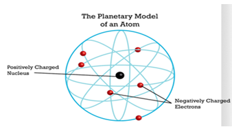
Figure 3.6 Planetary atomic model (Rutherford, 1911)

 

The Smallness of the Atom. Rutherford’s gold foil experiment was the first indication and proof that the space occupied by an atom is huge compared to that occupied by its nucleus. In fact, the electrons orbiting the nucleus can be compared to a few flies in a cathedral. As a qualitative reference, a human is about two million times “taller” than the average Escherichia coli bacterium; Mount Everest is about 5,000 times taller than the average man; and a man is about ten billion times “taller” than the oxygen atom. If the atom were scaled up to a size of a golf ball, on that same scale a man would stretch from Earth to the Moon. Atoms are so small that direct visualization of their structure is impossible. Today’s best optical or electron microscopes cannot reveal the interior of an atom.

The picture shown in figure 3.7 was taken with a scanning transmission electron microscope and shows a direct observation of cubes of magnesium oxide molecules, but details of the atoms cannot be seen.

 

 

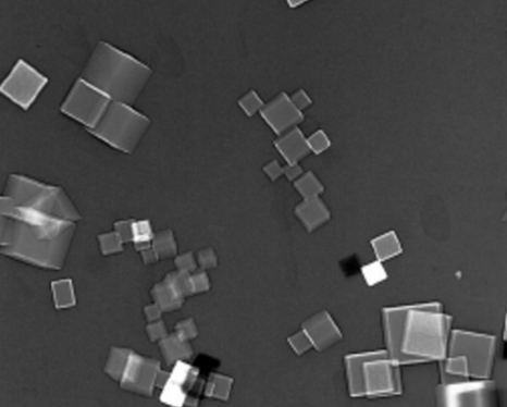
Figure 3.7 Magnesium oxide molecules as seen with scanning transmission electronic microscope produced at the Institute of Standards and Technology in the USA (Courtesy National Institute of Standards and Technology)

 

The image shown in figure 3.8 represents an 8 nm square structure with cobalt atoms arranged on a copper surface. Such arrangements of atoms are used to investigate the physics of ultra-tiny objects. The shown structure was observed with a scanning tunneling microscope at a temperature of 2.3 K (about −455º F): the larger peaks (upper left and lower right) are pairs of cobalt atoms, while the two smaller peaks are single cobalt atoms. The swirls on the copper surface illustrate how the cobalt and copper electrons interact with each other [13, p. 20].

 

 

Figure 3.8 Nanoscale structure of cobalt and copper atoms produced at the Institute of Standards and Technology in the USA (Courtesy of J. Stroscio, R. Celotta, A. Fein, E. Hudson, and S. Blankenship, 2002)

 

The Quantum Atomic Model. Quantum Leap.  In 1913, Niels Bohr (1885–1962) developed the atomic model that resolved Rutherford’s atomic stability questions. His model was based on the work of Planck (energy quantization), Einstein (photon nature of light) and Rutherford (nucleus at the center of the atom).

In 1900, Max Planck (1858–1947) resolved the long-standing problem of black body radiation by showing that atoms emit light in bundles of radiation (called photons by Einstein in 1905 in his theory of the photoelectric effect). This led to formulation of Planck’s radiation law: a light is emitted as well as absorbed in discrete quanta of energy. The magnitude of these discrete energy quanta is proportional to the light’s frequency (f, which represents the color of light) (1):

 

E = hf =  hc/𝜆 (1)

 

where h is Planck’s constant (h = 6.63 × 10−34 J s), c is the speed of light and λ is the wavelength of the emitted or absorbed light. Bohr applied this quantum theory of light to the structure of the electrons by restricting them to exist only along certain orbits (called the allowed orbits) and not allowing them to appear at arbitrary locations inside the atom. The angular momentum of the electrons is quantized and thus prohibits random trajectories around the nucleus. Consequently the electrons cannot emit or absorb electromagnetic radiation in arbitrary amounts since an arbitrary amount would lead to an energy that would force the electron to move to an orbit that does not exist. Electrons are thus allowed to move from one orbit to another. However, the electrons never actually cross the space between the orbits. They simply appear or disappear within the allowed states; a phenomenon referred to as a quantum leap or quantum jump.

For his theory of atoms that introduced the new discipline of quantum mechanics in physics, Bohr received a Noble Prize in 1922. He was also a founder of the Copenhagen school of quantum mechanics. One of his students once noticed a horseshoe nailed above his cabin door and asked him: “Surely, Professor Bohr, you don’t believe in all that silliness about the horseshoe bringing good luck?” With a gentle smile Bohr replied, “No, no, of course not, but I understand that it works whether you believe it or not” [13, p. 21].

 

Atoms of Higher Z. Quantum Numbers. The light spectra of atoms with more than one electron are much more complex than that of the hydrogen atom (many more lines). The calculations of the spectra for these atoms with the Bohr atomic model are complicated by the screening effect of the other electrons. Examination of the hydrogen spectral lines with high-resolution spectroscopes shows these lines to have very fine structures, and the observed spectral lines are each actually made up of several lines that are very close together. This observation implied the existence of sublevels of energy within the principal energy level, which makes Bohr’s theory inadequate even for the hydrogen atomic spectrum.

Bohr recognized that the electrons are most likely organized into orbital groups in which some are close and tightly bound to the nucleus, and others less tightly bound at larger orbits. He proposed a classification scheme that groups the electrons of multi-electron atoms into “shells” and each shell corresponds to a so-called quantum number n. These shells are given names that correspond to the values of the principal quantum numbers:

·         n = 1 (K shell) can hold no more than 2 electrons

·         n = 2 (L shell) can hold no more than 8 electrons

·         n = 3 (M shell) can hold no more than 18 electrons, etc.

 

Moseley’s work contributed to the understanding that the electrons in an atom existed in groups visualized as electron shells, and according to quantum mechanics, the electrons are distributed around the nucleus in probability regions also called the atomic orbitals.

 

In order to completely describe an atom in three dimensions, Schrödinger introduced three quantum numbers in addition to the principal quantum number, n. There are thus a total of four quantum numbers that specify the behavior of electrons in an atom, namely

·         principal quantum number, n = 1, 2, 3, …

·         azimuthal quantum number, l = 0 to n – 1

·         magnetic quantum number, m = −l to 0 to +l

·         spin quantum number, s = −1/2 or +1/2.

 

The principal quantum number describes the shells in which the electrons orbit. The maximum number of electrons in a shell n is 2n².

 

   The sub-energy levels (s, p, d, etc.) are the reason for the very fine structure of the spectral lines and result from the electron’s rotation around the nucleus along elliptical (not circular) orbits.

 

The azimuthal quantum number describes the actual shape of the orbits.

 

For example, l = 0 refers to a spherically shaped orbit, l = 1 refers to two obloid spheroids tangent to one another and l = 2 indicates a shape that is quadra-lobed (similar to a four leaf clover). For a given principal quantum number, n, the maximum number of electrons in an l = 0 orbital is 2, for an l = 1 orbital it is 6 and an l = 2 orbital can accommodate a maximum of 10 electrons.

 

The magnetic quantum number is also referred to as the orbital quantum number and it physically represents the orbital’s direction in space. For example when l = 0, m can only be zero. This single value for the magnetic quantum number suggests a single spatial direction for the orbital. A sphere is uni-directional and it extends equally in all directions, thus the reason for a single m value. If l = 1 then m can be assigned the values −1, 0 or +1. The three values for m suggest that the double-lobed orbital has three distinctly different directions in three-dimensional space into which it can extend. In the absence of any perturbing force (such could be an external magnetic field) the orbitals with the same n and l are equal in energy and are called degenerate.

 

 

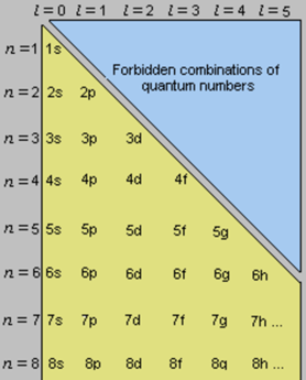
Figure 3.9 Allowed combinations of quantum numbers

 

In the presence of a perturbing force caused by the magnetic field the orbitals would differ in energy, and thus this quantum number is called the magnetic quantum number.

The spin quantum number describes the spin of the electrons. The electrons spin around an imaginary axis (as Earth spins about the imaginary axis connecting the north and south poles) in a clockwise or counterclockwise direction; for this reason there are two values, −1/2 or +1/2. The allowed combination of quantum numbers is given in figure 3.9 [13, p. 39].

 

The Wave Nature of Light.  If you drop a stone into one end of a quiet pond, the impact of the stone with the water starts an up-and-down motion of the water surface. This up-and-down motion travels outward from where the stone hit; it is a familiar example of a wave. A wave is a continuously repeating change or oscillation in matter or in a physical field. Light is also a wave. It consists of oscillations in electric and magnetic fields that can travel through space. Visible light, x rays, and radio waves are all forms of electromagnetic radiation.

You characterize a wave by its wavelength and frequency. The wavelength, denoted by the Greek letter λ (lambda), is the distance between any two adjacent identical points of a wave. Thus, the wavelength is the distance between two adjacent peaks or troughs of a wave. figure 3.3 shows a cross section of a water wave at a given moment, with the wavelength (λ) identified. Radio waves have wavelengths from approximately 100 mm to several hundred meters. Visible light has much shorter wavelengths, about 10^-6m. Wavelengths of visible light are often given in nanometers (1 nm = 10^-9 m). For example, light of wavelength 5.55 ∙ 10^-7 m, the greenish yellow light to which the human eye is most sensitive, equals 555 nm.

The frequency of a wave is the number of wavelengths of that wave that pass a fixed point in one unit of time (usually one second). For example, imagine you are anchored in a small boat on a pond when a stone is dropped into the water. Waves travel outward from this point and move past your boat. The number of wavelengths that pass you in one second is the frequency of that wave. Frequency is denoted by the Greek letter v (nu, pronounced “new”). The unit of frequency is /s, or s^-1, also called the hertz (Hz).

The wavelength and frequency of a wave are related to each other. figure 3.4 shows two waves, each traveling from left to right at the same speed; that is, each wave moves the same total length in 1s. The top wave, however, has a wavelength twice that of the bottom wave. In 1s, two complete wavelengths of the top wave move left to right from the origin. It has a frequency of 2/s, or 2 Hz. In the same time, four complete wavelengths of the bottom wave move left to right from the origin. It has a frequency of 4/s, or 4 Hz. Note that for two waves traveling with a given speed, wavelength and frequency are inversely related: the greater the wavelength, the lower the frequency, and vice versa. In general, with a wave of frequency v and wavelength λ, there are v wavelengths, each of length λ, that pass a fixed point every second. The product vλ is the total length of the wave that has passed the point in 1s. This length of wave per second is the speed of the wave. For light of speed c (2),

 

c = vλ (2)

 

The speed of light waves in a vacuum is a constant and is independent of wavelength or frequency. This speed is 3.00 ∙ 10⁸ m/s, which is the value for c that we use in the following examples. The range of frequencies or wavelengths of electromagnetic radiation is called the electromagnetic spectrum, shown in figure 3.5. Visible light extends from the violet end of the spectrum, which has a wavelength of about 400 nm, to the red end, with a wavelength of less than 800 nm. Beyond these extremes, electromagnetic radiation is not visible to the human eye. Infrared radiation has wavelengths greater than 800 nm (greater than the wavelength of red light), and ultraviolet radiation has wavelengths less than 400 nm (less than the wavelength of violet light) [15, p. 265].

 

Quantum Effects and Photons. Isaac Newton, who studied the properties of light in the seventeenth century, believed that light consisted of a beam of particles. In 1801, however, British physicist Thomas Young showed that light, like waves, could be diffracted. Diffraction is a property of waves in which the waves spread out when they encounter an obstruction or small hole about the size of the wavelength. You can observe diffraction by viewing a light source through a hole—for example, a streetlight through a mesh curtain. The image of the streetlight is blurred by diffraction.

By the early part of the twentieth century, the wave theory of light appeared to be well entrenched. But in 1905 the German physicist Albert Einstein (1879–1955; emigrated to the United States in 1933) discovered that he could explain a phenomenon known as the photoelectric effect by postulating that light had both wave and particle properties. Einstein based this idea on the work of the German physicist Max Planck (1858–1947) [15, p. 268].

 

Planck’s Quantization of Energy. In 1900 Max Planck found a theoretical formula that exactly describes the intensity of light of various frequencies emitted by a hot solid at different temperatures. Earlier, others had shown experimentally that the light of maximum intensity from a hot solid varies in a definite way with temperature. A solid glows red at 750_C, then white as the temperature increases to 1200ºC. At the lower temperature, chiefly red light is emitted. As the temperature increases, more yellow and blue light become mixed with the red, giving white light.

According to Planck, the atoms of the solid oscillate, or vibrate, with a definite frequency v, depending on the solid. But in order to reproduce the results of experiments on glowing solids, he found it necessary to accept a strange idea. An atom could have only certain energies of vibration, E, those allowed by the formula (3)

   

                                               E =  nhv, n =1, 2, 3, . . . (3)

 

where h is a constant, now called Planck’s constant, a physical constant relating energy and frequency, having the value 6.63 ∙ 10^-34J∙s. The value of n must be 1 or 2 or some other whole number. Thus, the only energies a vibrating atom can have are h_, 2h_, 3h_, and so forth.

The numbers symbolized by n are called quantum numbers. The vibrational energies of the atoms are said to be quantized; that is, the possible energies are limited to certain values.

The quantization of energy seems contradicted by everyday experience. Consider the potential energy of an object, such as a tennis ball. Its potential energy depends on its height above the surface of the earth: the greater the upward height, the greater the potential energy. (Recall the discussion of potential energy in Section 6.1.) We have no problem in placing the tennis ball at any height, so it can have any energy. Imagine, however, that you could only place the tennis ball on the steps of a stairway. In that case, you could only put the tennis ball on one of the steps, so the potential energy of the tennis ball could have only certain values; its energy would be quantized. Of course, this restriction of the tennis ball is artificial; in fact, a tennis ball can have a range of energies, not just particular values. As we will see, quantum effects depend on the mass of the object: the smaller the mass, the more likely you will see quantum effects. Atoms, and particularly electrons, have small enough masses to exhibit quantization of energy; tennis balls do not [15, p. 268].

 

Photoelectric Effect. Planck himself was uneasy with the quantization assumption and tried unsuccessfully to eliminate it from his theory. Albert Einstein, on the other hand, boldly extended Planck’s work to include the structure of light itself. Einstein reasoned that if a vibrating atom changed energy, say from 3h to 2h, it would decrease in energy by h, and this energy would be emitted as a bit (or quantum) of light energy. He therefore postulated that light consists of quanta (now called photons), or particles of electromagnetic energy, with energy E proportional to the observed frequency of the light (4):

                          

E = hv (4)

 

In 1905 Einstein used this photon concept to explain the photoelectric effect.

The photoelectric effect is the ejection of electrons from the surface of a metal or from another material when light shines on it (see figure 3.6). Electrons are ejected, however, only when the frequency of light exceeds a certain threshold value characteristic of the particular metal. For example, although violet light will cause potassium metal to eject electrons, no amount of red light (which has a lower frequency) has any effect.

To explain this dependence of the photoelectric effect on the frequency, Einstein assumed that an electron is ejected from a metal when it is struck by a single photon. Therefore, this photon must have at least enough energy to remove the electron from the attractive forces of the metal. No matter how many photons strike the metal, if no single one has sufficient energy, an electron cannot be ejected. A photon of red light has insufficient energy to remove an electron from potassium. But a photon corresponding to the threshold frequency has just enough energy, and at higher frequencies it has more than enough energy. When the photon hits the metal, its energy h is taken up by the electron. The photon ceases to exist as a particle; it is said to be absorbed.

The wave and particle pictures of light should be regarded as complementary views of the same physical entity. This is called the wave–particle duality of light. The equation E = hv displays this duality; E is the energy of a light particle or photon, and v is the frequency of the associated wave. Neither the wave nor the particle view alone is a complete description of light [15, p. 26].

 

Sizes of Atoms and Ions. In earlier chapters we discovered the importance of atomic masses in matters relating to stoichiometry. To understand certain physical and chemical properties, we need to know something about atomic sizes. In this section we describe atomic radius, the first of a group of atomic properties that we will examine in this chapter

 

Atomic Radius. The size of an atom, expressed as the atomic radius, represents the distance between the nucleus and the valence, or outermost, electrons. The boundary between the nucleus and the electrons is not easy to determine and the atomic radius is therefore approximated. For example, the distance between the two chlorine atoms of Cl₂ is known to be nearly 2Å. In order to obtain the atomic radius, the distance between the two nuclei is assumed to be the sum of the radii of two chlorine atoms. Therefore the atomic radius of chlorine is ~1Å (or 100 pm, see figure 3.10).

The atomic radius changes across the periodic table of elements and is dependent on the atomic number and the electron distribution. Since electrons repel each other due to like charges, the overall size of the atom increases with an increase in the number of electrons in each of the groups (see figure 3.10). For example, the radius of a hydrogen atom is smaller than the radius of the lithium atom. The outer electron of lithium is in the n = 2 level, so its radius must be larger than the radius of hydrogen which has its outermost electron in the n = 1 level. However, in spite of the increase in the number of electrons, the atomic radius decreases when going from left to right across the periodic table. This is a result of an increase in the number of protons for these elements, which all have their valence electrons in the same quantum energy level. Since the electrons are attracted to the protons, the increased charge of the nucleus (more protons) binds the electrons more tightly and brings them closer to the nucleus, causing the overall atomic radius to decrease. For example, the first two elements in the second period of the periodic table are lithium and beryllium.

 

 

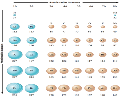
Figure 3.10 Trends of atomic radii (listed in picometers) in the periodic table

 

The radius of a beryllium atom is 113 pm, which is smaller than that of lithium (152 pm). In beryllium, Z = 4, the fourth electron joins the third in the 2s level, assuming their spins are anti-parallel. The charge is thus larger and this causes the electrons to be bound more tightly to the nucleus; as a result the beryllium radius is less than the lithium radius. The effect of the increased charge should, however, be seen in the context of the quantum energy levels. For example, cesium has a large number of protons but it is one of the largest atoms. The valence electrons are furthest from the nucleus and the inner electrons shield them from the positive charge of the nucleus; thus the valence electrons experience a reduced effective nuclear charge and not the total charge of the nucleus. The effect of the increase in the nuclear charge thus only plays a role in the periods from left to right, e.g., from sodium to argon in the third period, since the additional valence electrons (in the same quantum energy level) are exposed to a greater effective nuclear charge along the period [13, p. 49].

 

Ionic Radius. When a metal atom loses one or more electrons to formion, the positive nuclear charge exceeds the negative charge of the electrons in the resulting cation. The nucleus draws the electrons in closer, and, as a consequence, the following holds true.

Cations are smaller than the atoms from which they are formed.

For isoelectronic cations, the more positive the ionic charge, the smaller the ionic radius.

Anions are larger than the atoms from which they are formed. For isoelectronic anions, the more negative the charge, the larger the ionic radius [3, p.372].

 

Ionization Energy. In discussing metals, we talked about metal atoms losing electrons and thereby altering their electron configurations. But atoms do not eject electrons spontaneously. Electrons are attracted to the positive charge on the nucleus of an atom, and energy is needed to overcome that attraction. The more easily its electrons are lost, the more metallic an atom is considered to be. The ionization energy, I, is the quantity of energy a gaseous atom must absorb to be able to expel an electron. The electron that is lost is the one that is most loosely held.

Ionization energies are usually measured through experiments based on the photoelectric effect in which gaseous atoms at low pressures are bombarded with photons of sufficient energy to eject an electron from the atom. Here are two typical values.

 

Mg(g) → Mg⁺(g) + e^-                         I₁ = 738 kJ/mol

Mg⁺(g) →  Mg²⁺⁽g) + e^-          I₂ = 1451 kJ/mol

 

The symbol l₁ stands for the first ionization energy the energy required to strip one electron from a neutral gaseous atom. I₂ is the second ionization energy - the energy to strip an electron from a gaseous ion with a charge of Further ionization energies are I₃, I₄,  and so on. Each succeeding ionization energy is invariably larger than the preceding one. In the case of magnesium, for example, in the second ionization, the electron, once freed, has to move away from an ion with a charge of +2 (Mg²⁺). More energy must be invested than for a freed electron to move away from an ion with a charge of +1(Mg⁺). This is a direct consequence of Coulomb s law, which states, in part, that the force of attraction between oppositely charged particles is directly proportional to the magnitudes of the charges.

Ionization energies decrease as atomic radii increase.

This observation that ionization energies decrease as atomic radii increase reflects the effect of n and Z_eff² on the ionization energy (I) (5).

                               

I= R_H × Z²_eff/n² (5)

 

so that across a period, as Z_eff increases and the valence-shell principal quantum number n remains constant, the ionization energy should increase. And down a group, as n increases and Z_eff increases only slightly, the ionization energy should decrease. Thus, atoms lose electrons more easily (become more metallic) as we move from top to bottom in a group of the periodic table [3, p. 374].

 

Magnetic Properties. An important property related to the electron configurations of atoms and ions is their behavior in a magnetic field. A spinning electron is an electric charge in motion. It induces a magnetic field (recall the discussion on page 334). In a diamagnetic atom or ion, all electrons are paired and the individual magnetic effects cancel out. A diamagnetic species is weakly repelled by a magnetic field. A paramagnetic atom or ion has unpaired electrons, and the individual magnetic effects do not cancel out. The unpaired electrons possess a magnetic moment that causes the atom or ion to be attracted to an external magnetic field. The more unpaired electrons present, the stronger is this attraction.

Manganese has a paramagnetism corresponding to five unpaired electrons, which is consistent with the electron configuration

 

Mn: [Ar]    

↑

↑

↑

↑

↑

↑↓

                3d                                                  4s

 

When a manganese atom loses two electrons, it becomes the ion Mn²⁺ which is paramagnetic, and the strength of its paramagnetism corresponds to five unpaired electrons.

 

Mn²⁺: [Ar]    

↑

↑

↑

↑

↑

                3d                                                   4s

 

When a third electron is lost to produce Mn³⁺, the ion has a paramagnetism corresponding to four unpaired electrons. The third electron lost is one of the unpaired 3d electrons [3, p. 379].

 

Mn³⁺: [Ar]    

↑

↑

↑

↑

                3d                                                   4s

 

Elements and Periodicity. The elements are found in various states of matter and define the independent constituents of atoms, ions, simple substances, and compounds. Isotopes with the same atomic number belong to the same element. When the elements are classified into groups according to the similarity of their properties as atoms or compounds, the periodic table of the elements emerges. Chemistry has accomplished rapid progress in understanding the properties of all of the elements. The periodic table has played a major role in the discovery of new substances, as well as in the classification and arrangement of our accumulated chemical knowledge. The periodic table of the elements is the greatest table in chemistry and holds the key to the development of material science. Inorganic compounds are classified into molecular compounds and solid-state compounds according to the types of atomic arrangements [14, p.1].

 

The origin of elements and their distribution. All substances in the universe are made of elements. According to the current generally accepted theory, hydrogen and helium were generated first immediately after the Big Bang, some 15 billion years ago. Subsequently, after the elements below iron (Z = 26) were formed by nuclear fusion in the incipient stars, heavier elements were produced by the complicated nuclear reactions that accompanied stellar generation and decay.

In the universe, hydrogen (77 %) and helium (21 %) are overwhelmingly abundant and the other elements combined amount to only 2%. Elements are arranged below in the order of their abundance,

 

¹₁H˃⁴₂He˃¹⁶₈O˃¹²₆C˃²⁰₁₄Ne˃²⁸₁₄Si˃²⁷₁₃Al˃²⁴₁₂Mg˃⁵⁶₂₆Fe

 

The atomic number of a given element is written as a left subscript and its mass number as a left superscript [14, p.6].

 

Discovery of elements. The long-held belief that all materials consist of atoms was only proven recently, although elements, such as carbon, sulfur, iron, copper, silver, gold, mercury, lead, and tin, had long been regarded as being atom-like. Precisely what constituted an element was recognized as modern chemistry grew through the time of alchemy, and about 25 elements were known by the end of the 18th century. About 60 elements had been identified by the middle of the 19th century, and the periodicity of their properties had been observed.

The element technetium (Z = 43), which was missing in the periodic table, was synthesized by nuclear reaction of Mo in 1937, and the last undiscovered element promethium (Z = 61) was found in the fission products of uranium in 1947. Neptunium (Z = 93), an element of atomic number larger than uranium (Z = 92), was synthesized for the first time in 1940. There are 103 named elements. Although the existence of elements Z = 104-111 has been confirmed, they are not significant in inorganic chemistry as they are produced in insufficient quantity.

All trans-uranium elements are radioactive, and among the elements with atomic number smaller than Z = 92, technetium, prometium, and the elements after polonium are also radioactive. The half-lives (refer to Section 7.2) of polonium, astatine, radon, actinium, and protoactinium are very short. Considerable amounts of technetium 99Tc are obtained from fission products. Since it is a radioactive element, handling 99Tc is problematic, as it is for other radioactive isotopes, and their general chemistry is much less developed than those of manganese and rhenium in the same group. Atoms are equivalent to alphabets in languages, and all materials are made of a combination of elements, just as sentences are written using only 26 letters [14, p.7].

 

Electronic structure of elements. Wave functions of electrons in an atom are called atomic orbitals. An atomic orbital is expressed using three quantum numbers; the principal quantum number, n; the azimuthal quantum number, l; and the magnetic quantum number, m_l. For a principal quantum number n, there are n azimuthal quantum numbers l ranging from 0 to n-1, and each corresponds to the following orbitals.

 

l : 0, 1, 2, 3, 4, …

    s, p, d, f, g, …

 

An atomic orbital is expressed by the combination of n and l. For example, n is 3 and l is 2 for a 3d orbital. There are 2l+1 m_l values, namely l, l-1, l-2, ..., -l. Consequently, there are one s orbital, three p orbitals, five d orbitals and seven f orbitals. The three aforementioned quantum numbers are used to express the distribution of the electrons in hydrogen-type atom, and another quantum number m_s (1/2, -1/2) which describes the direction of an electron spin is necessary to completely describe an electronic state.    Therefore, an electronic state is defined by four quantum numbers (n, l, m_l, m_s).

The wave function ψ which determines the orbital shape can be expressed as the product of a radial wave function R and an angular wave function Y as follows (6).

 

ψ_n,l,ml = R_n,l(r)Y_l,ml(θ,φ) (6)

 

R is a function of distance from the nucleus, and Y expresses the angular component of the orbital. Orbital shapes are shown in figure 3.11. Since the probability of the electron’s existence is proportional to the square of the wave function, an electron density map resembles that of a wave function. The following conditions must be satisfied when each orbital is filled with electrons.

 

Pauli principle: The number of electrons that are allowed to occupy an orbital must be limited to one or two, and, for the latter case, their spins must be anti-parallel (different direction).

 

Hund's rule: When there are equal-energy orbitals, electrons occupy separate orbitals are their spins are parallel (same direction).

 

The order of orbital energy of a neutral atom is

1s < 2s < 2p < 3s < 3p < 4s < 3d < 4p …

and the electron configuration is determined as electrons occupy orbitals in this order according to the Pauli principle and Hund's rule. An s orbital with one m_l can accommodate 2 electrons, a p orbital with three ml 6 electrons, and a d orbital with five ml 10 electrons.

C: 1s²2s²2p² or [He] 2s²2p²

Fe: 1s²2s²2p⁶3s²3p⁶3d⁶4s² or [Ar] 3d⁶4s²

Au: 1s² 2s² 2p⁶ 3s² 3p⁶ 3d¹⁰ 4s² 4p⁶ 4d¹⁰ 4f¹⁴ 5s² 5p⁶ 5d¹⁰ 6s¹ or [Xe] 4f¹⁴ 5d¹⁰ 6s¹ [14, p.7]

 

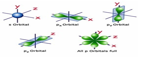
Figure 3.11 Shapes of s, p, and d orbitals.

 

The Aufbau Principle. The quantum numbers and the Pauli exclusion principle define the maximum number of the electrons that can be found in each of the electron orbits in an atom and also explain how the electrons are arranged. The aufbau principle (German meaning “to build up” thus also known as the building-up principle) explains the order in which the electrons occupy the orbitals. According to this principle the lowest energy orbitals in an atom are filled before those in the higher energy levels. Each orbital can accommodate at most two electrons (confirmed by spectroscopic and chemical analysis). According to additional rule, called the Hund’s rule, if two or more energetically equivalent orbitals are available (such as orbitals p, d, f) the electrons spread out before they start to pair. The reason for this is that because the electrons repel each other and because each orbital is directed toward a different section in space, the electrons can depart from each other. The Hund’s rule also says that the unpaired electrons in degenerate orbitals have the same spin alignment [13, p. 44].

 

Mendeleev’s Periodic Table. As previously described, the periodic table is a tabular arrangement of the elements that groups similar elements together. Mendeleev s work attracted more attention than Meyer’s for two reasons: He left blank spaces in his table for undiscovered elements, and he corrected some atomic mass values. The blanks in his table came at atomic masses 44, 68, 72, and 100 for the elements we now know as scandium, gallium, germanium, and technetium. Two of the atomic mass values he corrected were those of indium and uranium.

 

 

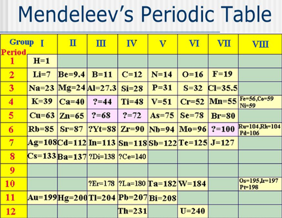
Figure 3.12 Mendeleev’s periodic table

 

In Mendeleev s table, similar elements fall in vertical groups, and the properties of the elements change gradually from top to bottom in the group. As an example, we have seen that the alkali metals (Mendeleev s group I) have high molar volumes (figure 3.13). They also have low melting points, which decrease in the order

 

Li (174 °C) ˃ Na (97.8 °C) ˃ K (63.7 °C) ˃ Rb (38.9 °C) ˃ Cs (28.5 °C)

 

In their compounds, the alkali metals exhibit the oxidation state +1, forming ionic compounds, such as NaCl, KBr, CsI, Li₂O, and so on [3, p.361].

 

Discovery of New Elements. Three elements predicted by Mendeleev were discovered shortly after the appearance of his 1871 periodic table (gallium, 1875; scandium, 1879; germanium, 1886). Table illustrates how closely Mendeleev s predictions for eka-silicon agree with the observed properties of the element germanium, discovered in 1886. Often, new ideas in science take hold slowly, but the success of Mendeleev s predictions stimulated chemists to adopt his table fairly quickly.

 

 

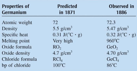
Figure 3.13 Comparison of the properties of Germanium as Predicted by Mendeleev and as Actually observed

 

One group of elements that Mendeleev did not anticipate was the noble gases. He left no blanks for them. William Ramsay, their discoverer, proposed placing them in a separate group of the table. Because argon, the first noble gas discovered (1894), had an atomic mass greater than that of chlorine and comparable to that of potassium, Ramsay placed the new group, which he called group 0, between the halogen elements (group VII) and the alkali metals (group I) [3, p.362].

 

The Periodic Table and Properties of the Elements. By the mid-19^th century, several chemists had discovered  that when the elements are arranged by atomic mass they demonstrate periodic behavior. In 1869, while writing a book on chemistry, Russian scientist Dmitri Mendeleev (1834–1907) realized this periodicity of the elements and he arranged them into a table that is today called the periodic table of elements. The table, as first published, was a simple observation of regularities in nature; the principles that defined this periodicity were not understood. Mendeleev’s table contained gaps due to the fact that some of the elements were yet unknown. In addition, when he arranged the elements in the table he noticed that the weights of several elements were wrong.

In the modern periodic table, the elements are grouped in order of increasing atomic number and arranged in rows (figure 3.14). Elements with similar physical and chemical properties appear in the same columns. A new row starts whenever the last (outer) electron shell in each energy level (principal quantum number) is completely filled. Properties of an element are discussed in terms of their chemical or physical characteristics. Chemical properties are often observed through a chemical reaction, while physical properties are observed by examining a pure element.

The chemical properties of an element are determined by the distribution of electrons around the nucleus, particularly the outer, or valence, electrons. Since a chemical reaction does not affect the atomic nucleus, the atomic number remains unchanged. For example, Li, Na, K, Rb and Cs behave chemically similarly because each of these elements has only one electron in its outer orbit. The elements of the last column (He, Ne, Ar, Kr, Xe and Rn) have filled inner shells and all except helium have eight electrons in their outermost shells. Because their electron shells are completely filled, these elements cannot interact chemically and are therefore referred to as the inert, or noble, gases.

 

 

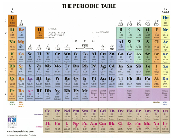
Figure 3.14 The periodic table of elements

 

Each horizontal row in the periodic table of elements is called a period. The first period contains only two elements, hydrogen and helium. The second and third periods each contain eight elements, while the fourth and fifth periods contain 18 elements each. The sixth period contains 32 elements that are usually arranged such that elements from Z = 58 to 71 are detached from main table and placed below it. The seventh and last period is also divided into two rows, one of which, from Z = 90 to 103, is placed below the second set of elements from the sixth period. The vertical columns are called groups and are numbered from left to right. The first column, Group 1, contains elements that have a closed shell plus a single s electron in the next higher shell. The elements in Group 2 have a closed shell plus two s electrons in the next shell. Groups 3–18 are characterized by the elements that have filled, or almost filled, p levels. Group 18 is also called Group 0 and contains the noble gases. The columns in the interior of the periodic table contain the transition elements in which the electrons are present in the d energy level. These elements begin in the fourth period because the first d level (3d) is in the fourth shell. The sixth and the seventh shells contain 4f and 5f levels and are called lanthanides, or rare earth elements, and actinides, respectively. The elements are also grouped according to their physical properties; for instance, they are grouped into metals, non-metals, and metalloids. Elements with very similar chemical properties are referred to as families; examples include the halogens, the inert gases, and the alkali metals. The following sections only focus on those atomic properties that are closely related to the principles of nuclear engineering [13, p. 45].

 

Block classification of the periodic table. Based on the composition of electron orbitals, hydrogen, helium and Group 1 elements are classified as s-block elements, Group 13 through Group 18 elements p-block elements, Group 3 through Group 12 elements d-block elements, and lanthanoid and actinoid elements f-block elements. s-Block, p-block, and Group 12 elements are called main group elements and d-block elements other than Group 12 and f-block elements are called transition elements. The characteristic properties of the elements that belong to these four blocks are described in Chapter 4 and thereafter. Incidentally, periodic tables that denote the groups of s-block and p-block elements with Roman numerals (I, II, ... , VIII) are still used, but they will be unified into the IUPAC system in the near future. Since inorganic chemistry covers the chemistry of all the elements, it is important to understand the features of each element through reference to the periodic table [14, p. 11].

 

Bonding states of elements. Organic compounds are molecular compounds that contain mainly carbon and hydrogen atoms. Since inorganic chemistry deals with all compounds other than organic ones, the scope of inorganic chemistry is vast. Consequently, we have to study the syntheses, structures, bonding, reactions, and physical properties of elements, molecular compounds, and solid-state compounds of 103 elements. In recent years, the structures of crystalline compounds have been determined comparatively easily by use of single crystal X-ray structural analysis, and by through the use of automatic diffractometers. This progress has resulted in rapid development of new areas of inorganic chemistry that were previously inaccessible. Research on higher dimensional compounds, such as multinuclear complexes, cluster compounds, and solid-state inorganic compounds in which many metal atoms and ligands are bonded in a complex manner, is becoming much easier. In this section, research areas in inorganic chemistry will be surveyed on the basis of the classification of the bonding modes of inorganic materials.

(a)   Element. Elementary substances exist in various forms. For example, helium and other rare gas elements exist as single-atom molecules; hydrogen, oxygen, and nitrogen as two-atom molecules; carbon, phosphorus, and sulfur as several solid allotropes; and sodium, gold, etc. as bulk metals. A simple substance of a metallic element is usually called bulk metal, and the word “metal” may be used to mean a bulk metal and “metal atom or metal ion” define the state where every particle is discrete. Although elementary substances appear simple because they consist of only one kind of element, they are rarely produced in pure forms in nature. Even after the discovery of new elements, their isolation often presents difficulties. For example, since the manufacture of ultra high purity silicon is becoming very important in science and technology, many new urification processes have been developed in recent years.

(b)   Molecular compounds. Inorganic compounds of nonmetallic elements, such as gaseous carbon dioxide CO₂, liquid sulfuric acid H₂SO₄, or solid phosphorus pentoxide P₂O₅, satisfy the valence requirements of the component atoms and form discrete molecules which are not bonded together. The compounds of main group metals such as liquid tin tetrachloride SnCl₄ and solid aluminum trichloride AlCl₃ have definite molecular weights and do not form infinite polymers.

Most of the molecular compounds of transition metals are metal complexes and organometallic compounds in which ligands are coordinated to metals. These molecular compounds include not only mononuclear complexes with a metal center but also multinuclear complexes containing several metals, or cluster complexes having metal-metal bonds. The number of new compounds with a variety of bonding and structure types is increasing very rapidly, and they represent a major field of study in today’s inorganic chemistry.

(c)    Solid-state compounds. Although solid-state inorganic compounds are huge molecules, it is preferable to define them as being composed of an infinite sequence of 1-dimensional (chain), 2-dimensional (layer), or 3-dimensional arrays of elements and as having no definite molecular weight. The component elements of an inorganic solid bond together by means of ionic, covalent, or metallic bonds to form a solid structure. An ionic bond is one between electronically positive (alkali metals etc.) and negative elements (halogen etc.), and a covalent bond forms between elements with close electronegativities. However, in many compounds there is contribution from both ionic and covalent bonds.

The first step in the identification of a compound is to know its elemental composition. Unlike an organic compound, it is sometimes difficult to decide the empirical formula of a solid-state inorganic compound from elemental analyses and to determine its structure by combining information from spectra. Compounds with similar compositions may have different coordination numbers around a central element and different structural dimensions. For example, in the case of binary (consisting of two kinds of elements) metal iodides, gold iodide, AuI, has a chain-like structure, copper iodide, CuI, a zinc blende type structure, sodium iodide, NaI, has a sodium chloride structure, and cesium iodide, CsI, has a cesium chloride structure, and the metal atoms are bonded to 2, 4, 6 or 8 iodine atoms, respectively. The minimum repeat unit of a solid structure is called a unit lattice and is the most fundamental information in the structural chemistry of crystals. X-ray and neutron diffraction are the most powerful experimental methods for determining a crystal structure, and the bonds between atoms can only be elucidated by using them. Polymorphism is the phenomenon in which different kinds of crystals of a solid-state compound are obtained in which the atomic arrangements are not the same. Changes between different polymorphous phases with variations in temperature and/or pressure, or phase transitions, are an interesting and important problem in solid-state chemistry or physics.

We should keep in mind that in solid-state inorganic chemistry the elemental composition of a compound are not necessarily integers. There are extensive groups of compounds, called nonstoichiometric compounds, in which the ratios of elements are non-integers, and these non-stoichiometric compounds characteristically display conductivity, magnetism, catalytic nature, color, and other unique solid-state properties. Therefore, even if an inorganic compound exhibits non-integral stoichiometry, unlike an organic compound, the compound may be a thermodynamically stable, orthodox compound. This kind of compound is called a non-stoichiometric compound or Berthollide compound, whereas a stoichiometric compound is referred to as a Daltonide compound. The law of constant composition has enjoyed so much success that there is a tendency to neglect non-stoichiometric compounds. We should point out that groups of compounds in which there are slight and continuous changes of the composition of elements are not rare [14, p. 12].